Using Administrative Data for Policy Evaluation

In-Person Workshop | ADR Evaluation Extension

Jake Anders, Oliver Cassagneau-Francis, Fabien Petit

UCL Centre for Education Policy & Equalising Opportunities

2026-09-17

Today

11:00	Welcome and setup	15 min
11:15	Analysing a cluster randomised trial	105 min
13:00	Lunch
13:45	Difference-in-differences with a policy reform	120 min
15:45	Break
16:00	Regression discontinuity, if we are on time	45 min
16:45	Wrap-up	15 min

This is a workshop focussed on implementation of the concepts discussed in the online modules.

• TIME — 2 min
• Set expectations early: nobody is expected to keep up with every line, and the code is all in the deck to take away
• Be straight about the third exercise: it is the flex block. It is self-contained and nothing later depends on it, so if the morning overruns we shorten or drop it rather than rushing the first two. Saying that up front stops it feeling like a failure if it happens
• The exercises are independent, so a participant who joins late or gets stuck in the morning can still start the afternoon clean

How we will work

The code is hidden by default. Every coding slide says what it is for; pick your own level, and change it slide by slide:

• Follow along — open the fold, run the code, work out what it did
• Read first — read the aim, predict what the code will do, then open the fold and run it
• Write your own — read the aim, write it yourself, open the fold to check

• Guided slides: on your own, at the pace on the screen
• “Your turn” tasks: with the person next to you, one keyboard, swap who types each task
• Discussions: in threes

If you are writing your own you will not finish every slide. Don’t worry — each exercise ends with a recap, and there are extensions in the appendix for anyone ahead.

• TIME — 2 min
• The three levels are self-selected and can change slide by slide — say so explicitly, people feel stuck otherwise
• Pairs for the tasks is deliberate: the audience is mostly students and analysts, and talking through a task fixes it better than typing it alone. One keyboard, so the pair actually talks
• Point at the appendix now so people know it exists. The extension slides are never presented; they are for anyone who is ahead, and for afterwards
• If the room is very mixed, suggest the proficient sit with someone who is not — it works better than proficient pairs racing ahead

Getting Set Up

What you should already have

1. R 4.1 or later, and RStudio or Positron/VSCode
2. The workshop project folder — everything is in it, including the data
3. The packages we will use:

install.packages(c("dplyr", "readr", "ggplot2", "fixest",
                   "modelsummary", "mice", "rdrobust", "rddensity"))

There is nothing to download and nothing to build. Open the project folder/file and you are ready.

• TIME — 2 min
• Run check-setup.R now if anyone has not already: this is the 15 minutes budgeted for it, and it should take seconds
• The setup is deliberately trivial this year. Earlier versions had participants download a 1.1 GB release from the UK Data Service and build the data on the day; an interrupted unzip then cost people the first half hour. Shipping simulated data removes that failure mode entirely
• rdrobust and rddensity are the only additions, both for the last exercise, and both are pure R — no compiler toolchain, so they install cleanly on a managed laptop
• Anyone still missing packages: get them installing now in the background, they only need the first two for the morning

How the code is written

We use	For
tidyverse where possible — readr, dplyr, tidyr, ggplot2, and the native pipe \|>	reading, reshaping, plotting
fixest::feols()	regression models
etable() at the console, modelsummary() for a report	regression tables
rdrobust, rddensity	regression discontinuity design
Two colours throughout: unaffected / control and affected / treatment	every plot

• Use whatever you are fluent in — the point is the estimand, not the syntax. But the folds and the solution scripts are written this way
• If a model call has no cluster =, the slide is about to show you why it needs one

Run this first, and again after lunch if you restart R:

library(dplyr); library(readr); library(ggplot2)
library(fixest); library(modelsummary)
theme_set(theme_minimal(base_size = 13))

• TIME — 4 min
• The library calls are on the slide because nothing else loads them: a participant who copies code from the slides into a fresh session needs to have run this once. Say it again after lunch
• Say the tidyverse choice out loud: it is the house style for the whole series, and a data.table user is welcome but will not get line-for-line matches with the folds
• read_csv rather than read.csv matters in the last exercise: it parses dates as dates. read.csv gives you a string and the running variable silently becomes nonsense
• The two colours are the same in every lecture deck and are colour-blind safe. Cyan is always the comparison group, purple always the treated group
• fixest because it is fast, clusters in the call, and its etable() reads well at a console. The modelsummary tables are what you would put in a report

Where this data comes from

No value here comes from LEO, and none describes a real person. They are constructed to resemble LEO and NPD data but as parameters you estimate were chosen as part of the simulation process.**

• It is simulated from scratch — there is no real extract underneath it, anonymised or otherwise
• What is borrowed is the shape: variable names, codings, formats, plausible distributions, and the awkward bits

• This means we know the right answer: the treatment effect, the intra-cluster correlation, the attrition patterns, etc., so we know what we’re aiming for
• It also means nothing here is a finding. Do not quote a number from today in anything!

• TIME — 3 min
• Say this early and plainly. This audience will work out what has been done, and it is much better coming from us
• Worth being explicit about why it is simulated rather than a real anonymised extract: anything genuinely derived from LEO could not be distributed like this, would need a licence and a download, and — because published synthetic releases are built by shuffling each column independently — would have no relationships left in it to teach with anyway
• The known-answer point is the one that actually sells it. You cannot check your own work against a real dataset, because nobody knows the true effect. Here we do
• If anyone wants the detail, variable-construction.csv in the project folder lists every column as simulated, reordered, imposed or constructed

The awkward bits are deliberate

Structural features	Target parameters
Variable names, codings and formats	The treatment effect, ICC and attrition rate
Plausible marginal distributions	The joint distribution between covariates
Missing-value patterns and text variables	Attainment 8 and post-16 destination
Unexpectedly text variables for numbers	The size of the discontinuity

These are realistic odd things about these admin data.

• TIME — 2 min
• These are not accidents and they are not us being unkind. Every one of them is a real feature of NPD and ILR extracts, and each has cost somebody a day of their life
• IDACI as a rank where 1 is MOST deprived catches almost everyone at least once — the sign of the coefficient comes out backwards and looks like a substantive finding
• The text sentinel sits in ethnic in all three pupil files. Nothing breaks when you summarise it; a factor conversion quietly gains a level, and a join on it silently drops those rows
• The right-hand column is the answer key, and it is the reason this beats practising on real data: nobody knows the true effect in a real dataset, so you cannot tell whether your analysis worked

Exercise 1: Analysing a Cluster RCT

The trial

A formative assessment programme delivered to whole schools. 140 secondary schools randomised 70/70, stratified by intake attainment and FSM share. Primary outcome: GCSE Attainment 8, linked from the National Pupil Database.

Modelled on Anders et al. (2022), the example used in Modules 1 and 2.

• Randomisation is at the school-level; the outcome is measured at the pupil-level
• The evaluation team generated the randomisation list; they were linked up with the NPD outcomes
• Protocol MDES was 0.18 SD

• TIME — 4 min
• Anchor this to Module 2: same estimand discussion, same clustering problem, same attrition questions, now in code
• The design is a real one and the numbers (140 schools, ICC 0.20, MDES 0.18 SD) are the real trial’s
• Stratified on intake attainment and FSM share — nine blocks, exactly as the real trial did. This matters later when we look at balance, and again when we put the blocks into the model

Load the trial data

pupils <- read_csv("data/trial_pupils.csv", show_col_types = FALSE)
schools <- read_csv("data/trial_schools.csv", show_col_types = FALSE)
rand <- read_csv("data/trial_randomisation.csv", show_col_types = FALSE)

dim(pupils)

#> [1] 25877    13

dim(schools)

#> [1] 138  11

dim(rand)

#> [1] 140   5

Three files. Which are from the evaluation team, and are the matches from the National Pupil Database?

glimpse(pupils)

#> Rows: 25,877
#> Columns: 13
#> $ pupil_id         <chr> "P000001", "P000002", "P000003", "P000004", "P000005", "P000006…
#> $ school_urn       <dbl> 125331, 125331, 125331, 125331, 125331, 125331, 125331, 125331,…
#> $ arm              <chr> "treatment", "treatment", "treatment", "treatment", "treatment"…
#> $ ks2_score        <dbl> 109, 98, 91, NA, 94, 115, 106, 106, 111, 109, 100, 108, 119, 11…
#> $ gender           <chr> "F", "M", "M", "M", "F", "F", "M", "F", "M", "F", "M", "F", "M"…
#> $ ethnic           <chr> "WBRI", "WBRI", "BAFR", "WBRI", "OOTH", "APKN", "WBRI", "WBRI",…
#> $ fsm6             <dbl> 0, 0, 0, 0, 1, 0, 0, 0, 0, 0, 0, 0, 0, 0, 0, 0, 0, 0, 0, 0, 0, …
#> $ sen_support      <dbl> 0, 0, 0, 0, 1, 0, 0, 0, 0, 0, 0, 0, 0, 0, 0, 0, 0, 0, 0, 1, 0, …
#> $ eal              <dbl> 0, 1, 0, 0, 0, 1, 1, 0, 0, 0, 0, 0, 0, 0, 0, 1, 0, 0, 1, 1, 0, …
#> $ idaci_rank       <dbl> 30313, 15780, 4710, 21568, 9114, 19065, 5446, 23083, 30487, 253…
#> $ attainment8      <dbl> 22, 34, 37, 38, 42, 82, 57, 49, 64, 65, 34, 46, 57, 68, 80, 68,…
#> $ destination_code <dbl> 120, 130, 110, 540, 130, 710, 220, 110, 220, 610, 130, 120, 120…
#> $ linked           <dbl> 1, 1, 1, 1, 1, 1, 1, 1, 1, 1, 1, 1, 1, 1, 1, 1, 1, 1, 1, 1, 1, …

• TIME — 2 min
• Three files for the morning, deliberately separate: the randomisation list is what the trial team held, the pupil records are what came back from the NPD, and the school frame is what you would assemble from Get Information About Schools
• Note 140 rows in the randomisation list and 138 schools in the pupil data. That is not a mistake and we come to it in a moment
• data/ also holds ilr_starts.csv and framework_lookup.csv for the afternoon, and npd_cohort.csv for the last exercise. Do not open them yet — the scenario lands better cold
• This slide sits inside Exercise 1 rather than in the setup on purpose: each exercise loads its own data, so anyone who restarts R can start any exercise from its first slide after the setup chunk

Does the data match the design?

Aim: count the schools in the randomisation list and in the pupil file, then list the schools that are in one but not the other, with their block and arm.

Before any analysis, check the file you were sent is the file you expected. What could explain a gap? Which explanations would be concerning?

nrow(rand) # schools randomised

#> [1] 140

n_distinct(pupils$school_urn) # schools with pupil records

#> [1] 138

anti_join(rand, pupils, by = "school_urn") |>
    select(school_urn, block, arm)

#> # A tibble: 2 × 3
#>   school_urn block                     arm      
#>        <dbl> <chr>                     <chr>    
#> 1     113849 mid attainment / high FSM treatment
#> 2     128542 mid attainment / high FSM treatment

• TIME — 6 min
• This is the single most valuable habit in the whole day. Two schools were randomised and never appear in the outcome data
• Ask the room what they think happened, before saying: they withdrew after randomisation
• The critical follow-up: does this break the trial? No — but it does mean the analysis sample is not the randomised sample, and it has to be reported. This is the top box of the CONSORT diagram
• Both withdrawing schools were treatment schools, in the same block. That is exactly the pattern to worry about: if treatment schools withdraw because the programme was burdensome, that is informative attrition. Two is too few to conclude anything, but you would want to know why

Checking balance

Aim: the mean of each baseline characteristic by arm, in one table.

Randomisation makes the arms comparable in expectation. Balance tables are how you show it worked this time. The rule for what goes in: measured before randomisation, or fixed.

pupils |>
    group_by(arm) |>
    summarise(
        n            = n(),
        `KS2 score`  = mean(ks2_score, na.rm = TRUE),
        `% FSM6`     = 100 * mean(fsm6),
        `% SEN`      = 100 * mean(sen_support),
        `% EAL`      = 100 * mean(eal),
        `IDACI rank` = mean(idaci_rank)
    ) |>
    mutate(across(where(is.numeric), \(x) round(x, 1)))

#> # A tibble: 2 × 7
#>   arm           n `KS2 score` `% FSM6` `% SEN` `% EAL` `IDACI rank`
#>   <chr>     <dbl>       <dbl>    <dbl>   <dbl>   <dbl>        <dbl>
#> 1 control   12478        104      28.7    13.5    20.7       16806.
#> 2 treatment 13399        104.     26      15.6    18.4       16236.

• TIME — 6 min
• Point out these are pre-randomisation characteristics only. Anything measured after randomisation cannot go in a balance table — it could have been affected by the treatment
• The arms look very similar. That is what stratifying on intake buys you
• Resist the urge to run a significance test on every row. A p-value here tests a null you already know is true by construction; large imbalances matter whether or not they are significant

Does balance need a test?

• The randomisation was random, so any imbalance is by definition chance
• What matters is not significance but magnitude: is the imbalance big enough to move the outcome?
• Adjust for (pre-specified) baseline covariates that strongly predict the outcome whether or not they look imbalanced — it buys precision

Pairs — 10 minutes

Add one more characteristic of your choice to the balance table — try gender, or the school-level pct_fsm6. Does anything look concerning?

• TIME — 10 min
• CONSORT explicitly discourages significance testing of baseline characteristics in randomised trials, and this is why
• Circulate. The common stumble is trying to add a school-level variable to a pupil-level summarise without joining first — which is a useful thing to hit
• Bring it back with: did anyone find something that worried them? Usually not, which is the point
• Pairs that finish early: the appendix extension on the pre-specified FSM subgroup uses the same join

Intention to treat: the analysis sample

Intention to treat. Compare pupils by the arm their school was assigned to, regardless of what the school actually did.

Aim: keep the pupils with an NPD record, and attach each school’s stratification block from the randomisation list.

analysis <- pupils |>
    filter(linked == 1) |>
    left_join(select(rand, school_urn, block), by = "school_urn")

nrow(analysis)

#> [1] 25336

• We drop only pupils with no NPD record at all — a linkage failure, not a treatment response
• We do not drop pupils whose school delivered the programme badly.
• That would be per-protocol, and it undermines randomisation. Use CACE/IV instead (not covered in this workshop).

• TIME — 4 min
• Straight callback to Module 2 Section 1. ITT preserves the randomisation; per-protocol conditions on a post-randomisation behaviour
• Worth stating the assumption per-protocol would need: that whether a school delivered well is unrelated to what its pupils would have scored anyway. Nobody believes that
• The 541 pupils we drop here are the linkage failures. We come back to whether that is safe
• The block join is for later: the trial stratified on it, so the analysis should use it

Unadjusted difference in means

Two things to notice in the call: the outcome, and cluster =. Why school?

m1 <- feols(attainment8 ~ arm, data = analysis, cluster = ~school_urn)
m1

#> OLS estimation, Dep. Var.: attainment8
#> Observations: 25,336
#> Standard-errors: Clustered (school_urn) 
#>              Estimate Std. Error   t value  Pr(>|t|)    
#> (Intercept)  45.66084    1.14567 39.855027 < 2.2e-16 ***
#> armtreatment  1.31436    1.54605  0.850142   0.39673    
#> ---
#> Signif. codes:  0 '***' 0.001 '**' 0.01 '*' 0.05 '.' 0.1 ' ' 1
#> RMSE: 18.7   Adj. R2: 0.00119

• TIME — 4 min
• cluster = ~school_urn from the very first model. Not an afterthought — the unit of randomisation is the school, so the unit of clustering is the school
• 1.31 Attainment 8 points, standard error 1.55, p = 0.40. On this evidence you would conclude the programme did nothing
• Ask: how big is 1.31 points? Nobody knows without the standard deviation, which is why we convert to effect sizes shortly

Add prior attainment

Aim: refit the model with KS2 prior attainment as a covariate.

Reminder: why are we including a baseline covariate in a randomised trial anyway? Not bias: randomisation handled that. It is there to soak up variation in the outcome that has nothing to do with the treatment. So useful baseline covariates predict the outcome strongly (sometimes called prognostic) and was measured before randomisation.

Which of these do you expect to change, and in which direction?

• estimate,
• standard error
• R²

m2 <- feols(attainment8 ~ arm + ks2_score,
    data = analysis,
    cluster = ~school_urn
)
m2

#> OLS estimation, Dep. Var.: attainment8
#> Observations: 24,663
#> Standard-errors: Clustered (school_urn) 
#>                Estimate Std. Error   t value  Pr(>|t|)    
#> (Intercept)  -137.86785   3.101478 -44.45231 < 2.2e-16 ***
#> armtreatment    1.99693   0.846617   2.35871  0.019751 *  
#> ks2_score       1.76468   0.028748  61.38375 < 2.2e-16 ***
#> ---
#> Signif. codes:  0 '***' 0.001 '**' 0.01 '*' 0.05 '.' 0.1 ' ' 1
#> RMSE: 14.1   Adj. R2: 0.442456

• TIME — 5 min
• Get answers to the prediction before opening the fold. The estimate should not move systematically (it is unbiased either way); the SE should fall a lot; R² should jump
• The estimate moves from 1.31 to 2.00 points, which is chance — both are unbiased. The standard error nearly halves, from 1.55 to 0.85
• That is the whole argument for covariate adjustment in one comparison: same target, far less noise
• Note 673 observations dropped for missing KS2. That is listwise deletion happening silently — flag it now, we return to it
• R-squared jumps from 0.001 to 0.44. Prior attainment is doing all the work

Add pupil characteristics and the blocks

Aim: add FSM6, SEN support and EAL as covariates, and the stratification blocks as fixed effects.

Once prior attainment is included, what must a covariate do to add precision? Will three demographics buy as much as prior attainment did?

Why should we include the stratification blocks?

m3 <- feols(attainment8 ~ arm + ks2_score + fsm6 + sen_support + eal | block,
    data = analysis, cluster = ~school_urn
)
m3

#> OLS estimation, Dep. Var.: attainment8
#> Observations: 24,663
#> Fixed-effects: block: 9
#> Standard-errors: Clustered (school_urn) 
#>              Estimate Std. Error   t value   Pr(>|t|)    
#> armtreatment  1.88677   0.804085   2.34648 2.0385e-02 *  
#> ks2_score     1.55190   0.023139  67.06892  < 2.2e-16 ***
#> fsm6         -6.29411   0.282203 -22.30349  < 2.2e-16 ***
#> sen_support  -6.63235   0.323425 -20.50661  < 2.2e-16 ***
#> eal           2.15896   0.524767   4.11413 6.6716e-05 ***
#> ---
#> Signif. codes:  0 '***' 0.001 '**' 0.01 '*' 0.05 '.' 0.1 ' ' 1
#> RMSE: 13.6     Adj. R2: 0.481451
#>              Within R2: 0.41864

• TIME — 4 min
• The answer to the prompt: it has to predict the outcome beyond what KS2 already explains. FSM, SEN and EAL are largely already reflected in prior attainment
• Another small gain: R-squared 0.44 to 0.48, standard error 0.85 to 0.80. Of that, the characteristics take it to 0.83 and the blocks the rest
• The blocks go in because the trial stratified on them — the real trial did exactly this. Analyse as you randomised
• The lesson is diminishing returns. This is worth saying explicitly because people often expect a long covariate list to help. It does not, and every extra covariate is another chance to lose observations to missingness

Three specifications, one table

Aim: the three models in one table — the treatment row only, with N and R².

Compare the standard errors.

modelsummary(
    ## Avoid a leading "+" in the names: markdown renders it as a bullet.
    list(
        "Unadjusted" = m1, "With prior attainment" = m2,
        "With characteristics and blocks" = m3
    ),
    coef_map = c("armtreatment" = "Treatment"),
    gof_map = c("nobs", "r.squared"),
    statistic = "({std.error})",
    stars = TRUE, output = "markdown"
)

	Unadjusted	With prior attainment	With characteristics and blocks
Treatment	1.314	1.997*	1.887*
	(1.546)	(0.847)	(0.804)
Num.Obs.	25336	24663	24663
R2	0.001	0.443	0.482
p < 0.1, * p < 0.05, ** p < 0.01, *** p < 0.001

• TIME — 4 min
• Read the standard error row across: 1.55, 0.85, 0.80
• The conclusion changes. Unadjusted, this trial found nothing. Adjusted, it found a clear positive effect
• This is not p-hacking, and it is important to say so: the covariates were pre-specified in the analysis plan before any outcome data was seen. Adjustment was always going to happen

The precision gain

Pairs — 15 minutes

Compute how much the standard error fell, and convert both estimates into effect sizes.

se_unadj <- ___   # from m1
se_adj   <- ___   # from m3
100 * (1 - se_adj / se_unadj)

sd_a8 <- sd(analysis$attainment8, na.rm = TRUE)

tibble(
    model     = c("Unadjusted", "Adjusted"),
    estimate  = c(coef(m1)[["armtreatment"]], coef(m3)[["armtreatment"]]),
    se        = c(se(m1)[["armtreatment"]], se(m3)[["armtreatment"]]),
    p         = c(pvalue(m1)[["armtreatment"]], pvalue(m3)[["armtreatment"]])
) |>
    mutate(
        effect_size = estimate / sd_a8,
        across(where(is.numeric), \(x) round(x, 3))
    )

#> # A tibble: 2 × 5
#>   model      estimate    se     p effect_size
#>   <chr>         <dbl> <dbl> <dbl>       <dbl>
#> 1 Unadjusted     1.31 1.55  0.397       0.07 
#> 2 Adjusted       1.89 0.804 0.02        0.101

• TIME — 15 min
• 48% reduction in the standard error. Equivalently, you would have needed well over three times as many schools to get this precision without adjusting
• Effect sizes: 0.07 SD unadjusted, 0.10 SD adjusted, against a protocol MDES of 0.18 SD
• Sit with that for a moment. The trial was designed to detect 0.18 SD and the estimate is smaller than that — yet it is statistically significant, because adjustment delivered more precision than the power calculation assumed
• Pairs that finish early: the appendix has the same-sample check (are m1 and m3 even fitted on the same pupils?)

Why clustering matters here

Aim: refit the adjusted model with plain (iid) standard errors, and put it beside the clustered one.

Which of the estimate and the standard error will change?

naive <- feols(attainment8 ~ arm + ks2_score + fsm6 + sen_support + eal | block,
    data = analysis, vcov = "iid"
)

modelsummary(
    list("Ignoring clustering" = naive, "Clustered by school" = m3),
    coef_map = c("armtreatment" = "Treatment"),
    gof_map = "nobs", statistic = "({std.error})", output = "markdown"
)

	Ignoring clustering	Clustered by school
Treatment	1.887	1.887
	(0.174)	(0.804)
Num.Obs.	24663	24663

• Same estimate. Very different standard error.

• TIME — 4 min
• The point estimate is identical to the last decimal. Clustering is an inference problem, not an estimation problem — exactly as Module 2 Section 3 said
• The naive standard error is far too small, because it treats 25,000 pupils as 25,000 independent observations when they sit in 138 schools sharing teachers, intake and the treatment itself
• Ask what the consequence would be: you would report a much smaller p-value and a much narrower confidence interval than you are entitled to

Intra-cluster correlation and the design effect

Aim: estimate the intra-cluster correlation (ICC) of Attainment 8 — the share of its variance that sits between schools — from a one-way ANOVA on school; then the design effect.

icc <- analysis |>
    filter(!is.na(attainment8)) |>
    (\(d) {
        fit <- lm(attainment8 ~ factor(school_urn), data = d)
        ms <- anova(fit)[["Mean Sq"]]
        nbar <- nrow(d) / n_distinct(d$school_urn)
        vb <- (ms[1] - ms[2]) / nbar
        vb / (vb + ms[2])
    })()

round(icc, 3)

#> [1] 0.199

round(1 + (nrow(analysis) / n_distinct(analysis$school_urn) - 1) * icc, 1)

#> [1] 37.3

• ICC around 0.20, average cohort about 185 pupils
• Design effect near 37 — 25,000 pupils providing roughly the information of 680 independent ones
• Could also estimate the ICC with a hierarchical model - keeping required packages to a minimum!

• TIME — 4 min
• Say what the ICC is in words before the number: if you know which school a pupil is in, how much do you know about their score? 0.20 means a fifth of the variance is between schools
• This is the number that explains everything about cluster trials. It is why you need 140 schools rather than 140 pupils
• ICC 0.20 is realistic for GCSE attainment in England and is what the real trial assumed at design stage
• The design effect is startling when you first see it. Let it land
• The practical implication: adding more pupils per school buys almost nothing. Adding schools is what buys power

Small numbers of clusters

• Cluster-robust standard errors are asymptotic in the number of clusters, not the number of pupils
• With 138 schools we are comfortable. Below roughly 30–40, they over-reject — a theoretically 5% test can reject 15% of the time
• Alternative methods such as wild cluster bootstrap (not done here)

Pairs — 10 minutes

Re-estimate m3 on a subset of just 20 schools. What happens to the standard error, and would you trust the p-value?

set.seed(1)
few <- analysis |>
    filter(school_urn %in% sample(unique(analysis$school_urn), 20))

feols(attainment8 ~ arm + ks2_score + fsm6 + sen_support + eal | block,
    data = few, cluster = ~school_urn
) |>
    coeftable() |>
    (\(x) round(x["armtreatment", ], 3))()

#>   Estimate Std. Error    t value   Pr(>|t|) 
#>      0.193      2.548      0.076      0.941

• TIME — 12 min
• The honest answer to “would you trust it”: the standard error is roughly right, but the p-value leans optimistic because the reference distribution is wrong with few clusters
• fwildclusterboot::boottest() is the standard tool. We are not running it live because it needs a compiler toolchain and we would lose people to installation problems
• Real cases where this bites: trials randomised at local authority level, where you might have 12 clusters
• Connect back to Module 2’s simulation — with unequal cluster sizes, cluster-robust standard errors still over-reject at 16% with six clusters
• Pairs that finish early: the appendix has randomisation inference, which needs no asymptotics at all

Attrition: how much, and is it differential?

Aim: for each arm, the number of pupils with no linked outcome and the share.

Which important things about attrition does this table tell us?

What important thing about attrition does it not tell us?

pupils |>
    group_by(arm) |>
    summarise(
        n = n(),
        not_linked = sum(linked == 0),
        pct = round(100 * mean(linked == 0), 2)
    )

#> # A tibble: 2 × 4
#>   arm           n not_linked   pct
#>   <chr>     <int>      <int> <dbl>
#> 1 control   12478        245  1.96
#> 2 treatment 13399        296  2.21

• TIME — 3 min
• 1.96% versus 2.21%. Overall attrition is low and it is not differential by arm (p ≈ 0.17) — which is the question that actually matters for internal validity
• Low overall missingness is the great advantage of administrative outcomes. A survey-based trial would be looking at 20-30% here
• But do not stop at this table. The rate being similar does not mean the missing pupils are a random subset — that is the question it does not answer

Who is missing?

Aim: baseline means for linked and unlinked pupils, side by side.

If the two groups differ, what is threatened — and does the answer depend on whether they also differ by arm?

pupils |>
    group_by(linked) |>
    summarise(
        n = n(),
        ks2 = round(mean(ks2_score, na.rm = TRUE), 1),
        pct_fsm6 = round(100 * mean(fsm6), 1),
        pct_sen = round(100 * mean(sen_support), 1),
        pct_eal = round(100 * mean(eal), 1)
    )

#> # A tibble: 2 × 6
#>   linked     n   ks2 pct_fsm6 pct_sen pct_eal
#>    <dbl> <int> <dbl>    <dbl>   <dbl>   <dbl>
#> 1      0   541  104.     32.7    16.3    27.4
#> 2      1 25336  104.     27.2    14.6    19.4

• TIME — 4 min
• Now the picture changes. Unlinked pupils are clearly more likely to be FSM-eligible (33% against 27%) and EAL (27% against 19%); SEN barely differs
• So attrition is non-random but not differential by arm. Those are different things and the distinction is the teaching point
• Non-random but balanced attrition threatens generalisability — who the result applies to — rather than internal validity. The estimate is still unbiased for the pupils you observe
• Had it been differential by arm as well, we would have a real problem, and the estimate could not be trusted

What to do about missing outcomes

• Primary specification: complete cases with covariate adjustment. Under missing-at-random given the covariates already in the model, this is unbiased and needs nothing extra
• Multiple imputation as a sensitivity analysis especially when there are additional predictors of missingness not in the analysis model
• Impute separately by arm, or at minimum include treatment and its interactions

• Do not forget missing values int he baseline, too: 673 pupils have no KS2 score and are silently dropped by every adjusted model above

• TIME — 4 min
• This reverses what people expect. MI is often presented as the responsible default and complete cases as lazy; for missing outcomes in a covariate-adjusted trial analysis that is backwards
• The missing KS2 is the one people miss. Those 673 pupils are in the unadjusted model and out of the adjusted one, so the two models are fitted on different samples
• For missing baseline covariates in a randomised trial, the missing indicator method is unbiased and simpler than imputation — the one place where the simple method genuinely wins
• mice runs in a couple of seconds on this data; it is in the appendix as an extension, imputing the missing KS2 with arm in the imputation model, and it changes nothing — which is the point

Interpreting this for a funder

What we found: an effect of about 0.10 SD on Attainment 8, clearly distinguishable from zero once we adjust for prior attainment, and estimated on 138 schools with 2.1% missing outcomes.

• Is 0.10 SD big? Roughly a month of additional progress — modest, but comparable to many things schools spend money on
• The trial was designed to detect 0.18 SD. We found something smaller and still called it significant — because adjustment gave us more precision than the design assumed
• The unadjusted analysis would have reported no strong evidence. Importantly the specification with prior attainment covariates was pre-specified.

• TIME — 5 min
• This is the discussion slot. Push the room: what would you actually write in the executive summary?
• The honest answer includes all three of: the effect size, the precision, and the fact that the headline depends on a pre-specified adjustment
• Cost is the missing dimension. A 0.10 SD effect from a cheap programme is very different from the same effect from an expensive one
• Good closing question: what would you want to know before recommending this programme further?

What you actually recovered

Because we built this dataset, we know the right answers:

	We set	You estimated
Treatment effect	0.10 SD	0.10 SD adjusted; 0.07 SD unadjusted
ICC	0.20	0.20
Attrition	~2%, non-differential	1.96% vs 2.21%

• The adjusted estimate recovers the simulated ‘truth’. The unadjusted one is 30% lower and non-significant by chance alone (both are unbiased) but that chance is higher without adjustment because the standard error is bigger.
• Reported without its pre-specified adjustment, this trial would have been reported as a null finding. Same data, same truth.

• TIME — 4 min
• Do this reveal properly, it is the payoff for the whole morning and it is only possible because the data is constructed
• The unadjusted shortfall is sampling noise, not a bug. With a standard error of 0.08 SD, an estimate of 0.07 against a truth of 0.10 is well inside one standard error. The adjusted estimate, with a standard error of 0.04 SD, could equally have landed at 0.06 or 0.14
• That is the general point: every published estimate is one draw from a sampling distribution, and the significant ones are drawn from its upper part when power is low — the winner’s curse. Landing on the truth this time is luck, not skill
• Good bridge to the afternoon: in the RCT we knew the assignment was random. After lunch we have to argue for it

Exercise 1: what you did

• Checked the data you were sent matched the design: found two schools missing
• Built a balance table and discussed whether it needs significance tests
• Estimated an intention-to-treat effect and showed how pre-specified adjustment can change the conclusion
• Clustered at the level of randomisation, and saw the consequences of ignoring that
• Distinguished attrition that is non-random from attrition that is differential

If you are ahead — four extensions in the appendix: the pre-specified FSM subgroup, multiple imputation with mice, randomisation inference, and whether the models are even on the same sample.

• TIME — 1 min
• Ninety seconds. The point is the shape: work out what you are estimating, check the design held, estimate it, then attack your own result
• Anyone who is ahead has the appendix; the rest of us go to lunch

Exercise 2: Difference-in-Differences

The reform

The SASE reform, August 2012. From that date, every new apprenticeship framework had to last at least 12 months and include at least 280 guided learning hours.

Frameworks already meeting those thresholds were unaffected. Frameworks below them had to change.

• That gives us a comparison group defined by the policy itself — not by our choice
• Outcomes: how many people start, whether they complete, whether they achieve, and what they earn afterwards
• Modelled on Nafilyan & Speckesser (2019), using ILR-style records 2008/09–2015/16

• TIME — 6 min
• The design logic: a national reform with no phase-in, so there is no staggered adoption to worry about and a plain two-way fixed effects model is appropriate. We return to that in the robustness section
• Why this is a good natural experiment: which frameworks were affected was determined by their pre-existing duration, not by anyone choosing to be treated
• Why it is not perfect: affected frameworks were systematically shorter, and shorter frameworks sit in different sectors. We look at that directly
• Eight years of data, four either side. A four-year window gives only one pre-reform coefficient, which is not enough to assess parallel trends

The ILR starts file

starts <- read_csv("data/ilr_starts.csv", show_col_types = FALSE)
dim(starts)

#> [1] 120001     19

names(starts)

#>  [1] "learner_id"              "framework_id"            "academic_year"          
#>  [4] "start_year"              "sex"                     "ethnicity"              
#>  [7] "lldd"                    "prior_attain"            "age_at_start"           
#> [10] "start_date"              "expected_end_date"       "planned_duration_months"
#> [13] "guided_learning_hours"   "compstatus"              "outcome"                
#> [16] "completion"              "achievement"             "earnings_12m"           
#> [19] "main_sic_section"

What is not in this file that the design needs?

• TIME — 4 min
• 120,000 individual apprenticeship starts, one row per learner per aim
• The answer: no ready-made treatment indicator, and no framework-level duration. Deriving those is the first task
• ethnicity, lldd and prior_attain carry raw ILR codes rather than labels. That is authentic and mildly annoying, which is the point

Who was affected?

Pairs — 10 minutes

The reform applied to frameworks whose planned duration was under 12 months before August 2012. Work out which frameworks those are, using only pre-reform starts.

framework_pre <- starts |>
    filter(start_year < 2012) |>
    group_by(framework_id) |>
    summarise(duration_pre = mean(planned_duration_months), .groups = "drop") |>
    mutate(affected = as.integer(duration_pre < 12))

count(framework_pre, affected)

#> # A tibble: 2 × 2
#>   affected     n
#>      <int> <int>
#> 1        0    38
#> 2        1    42

• TIME — 14 min
• The key discipline: define treatment using PRE-reform data only. Using all years would let the reform itself determine who counts as treated, which is circular
• 42 affected, 38 unaffected — a comfortable split
• Ask why we take a mean rather than a single value: individual aims vary around the framework’s planned duration, so we need the framework-level central tendency
• The 12-month threshold is sharp in policy but fuzzy in data. Anyone who plots the distribution will see frameworks sitting close to the line — a good prompt for whether a regression discontinuity would suit better
• Pairs that finish early: plot the distribution of duration_pre with a line at 12

First stage: did planned durations change?

Aim: mean planned duration by affected group and start year, as a line plot with the reform marked.

What must this plot show before any effect estimate is believable?

starts |>
    left_join(framework_pre, by = "framework_id") |>
    group_by(start_year, affected = factor(
        affected, 0:1,
        c("Unaffected", "Affected")
    )) |>
    summarise(duration = mean(planned_duration_months), .groups = "drop") |>
    ggplot(aes(start_year, duration, colour = affected)) +
    geom_vline(xintercept = 2011.5, linetype = "dashed", colour = "grey50") +
    geom_hline(yintercept = 12, linetype = "dotted", colour = "grey50") +
    geom_line(linewidth = 1) +
    geom_point(size = 2) +
    scale_colour_manual(values = c(Unaffected = "#30d6ff", Affected = "#993bff")) +
    labs(x = NULL, y = "Mean planned duration (months)", colour = NULL)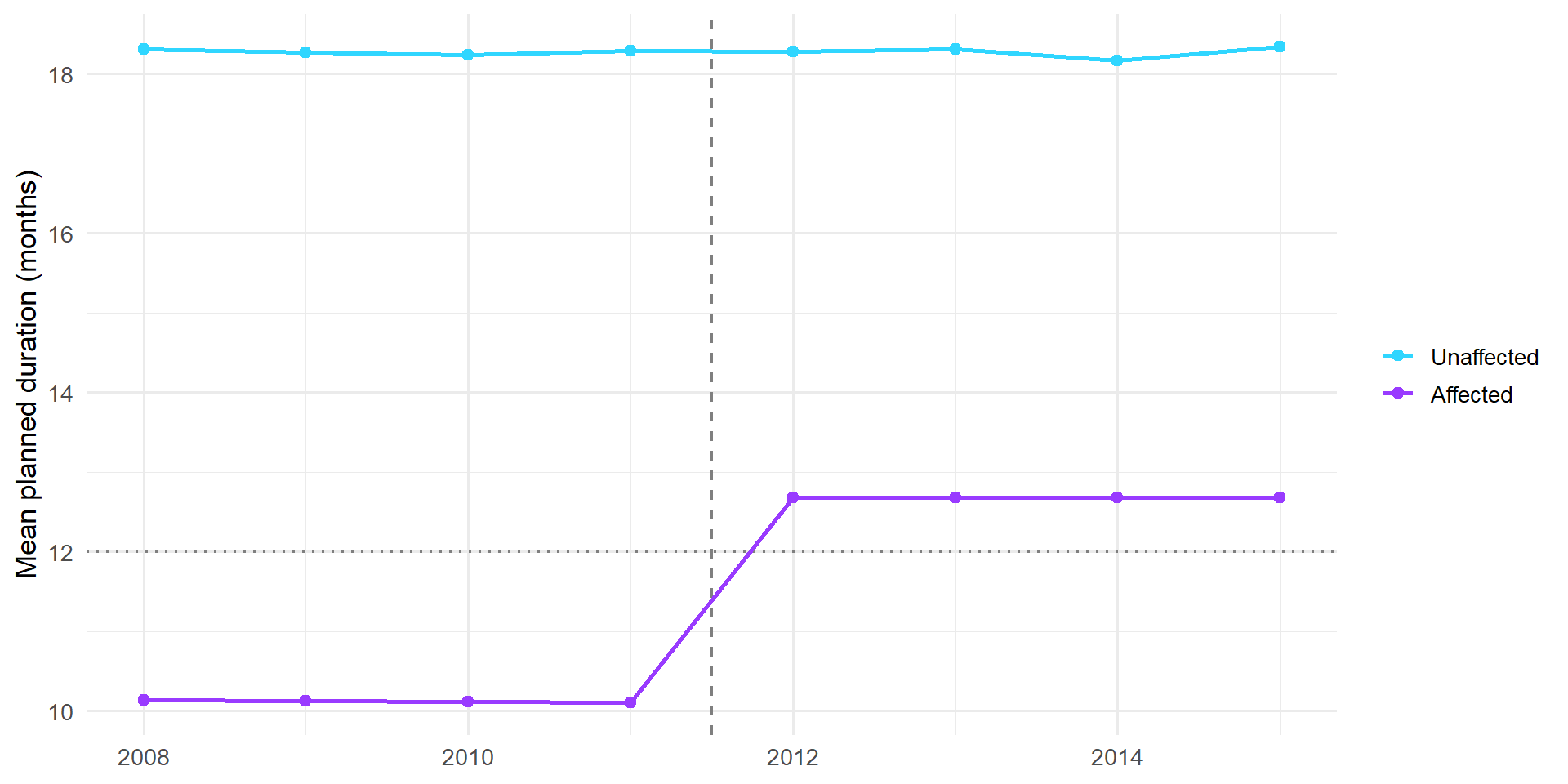

• TIME — 6 min
• This is the first stage, and it is the most convincing slide of the afternoon. Affected frameworks jump from about 10 months to nearly 13 in 2012/13; unaffected frameworks do not move at all
• Always show this before showing effects. If the policy did not change behaviour, there is nothing to attribute an outcome change to
• Ask the room what they would conclude if the affected line had drifted upwards from 2010. Answer: anticipation, and the clean before-and-after comparison would be in trouble

Build the analysis panel

Aim: attach affected to every start, flag post-reform starts and their interaction, then collapse to one row per framework × year: the number of starts, the completion and achievement rates, the mean of log earnings among completers — and how many completers that mean is over.

Why aggregate at all, and what does a cell mean hide?

panel <- starts |>
    left_join(framework_pre, by = "framework_id") |>
    mutate(
        post = as.integer(start_year >= 2012),
        did = affected * post
    ) |>
    group_by(framework_id, start_year, affected, post, did) |>
    summarise(
        starts = n(),
        completion = mean(completion),
        achievement = mean(achievement),
        n_earn = sum(!is.na(earnings_12m)),
        log_earn = mean(log(earnings_12m), na.rm = TRUE),
        .groups = "drop"
    )

dim(panel)

#> [1] 640  10

• TIME — 10 min
• 80 frameworks by 8 years = 640 cells, fully balanced
• We aggregate because the policy applies to frameworks, not individuals, and starts only exist as a count at that level. The clustering is what matters and there are only 80 clusters either way
• What a cell mean hides: how many people are behind it. n_earn is kept for exactly that reason — the earnings cells range from a few dozen completers to several hundred, and the reform changed those counts differentially. We come back to it when we fit the earnings model
• did = affected * post written explicitly rather than relying on interaction syntax — clearer, and it is what goes in the model
• About 12% of completers have no PAYE record; they are simply not in n_earn or log_earn

Parallel trends, by eye

Aim: the completion rate by group and start year, plotted.

Write one sentence assessing the pre-period before the next slide.

panel |>
    group_by(start_year, affected = factor(
        affected, 0:1,
        c("Unaffected", "Affected")
    )) |>
    summarise(completion = mean(completion), .groups = "drop") |>
    ggplot(aes(start_year, completion, colour = affected)) +
    geom_vline(xintercept = 2011.5, linetype = "dashed", colour = "grey50") +
    geom_line(linewidth = 1) +
    geom_point(size = 2) +
    scale_colour_manual(values = c(Unaffected = "#30d6ff", Affected = "#993bff")) +
    labs(x = NULL, y = "Completion rate", colour = NULL)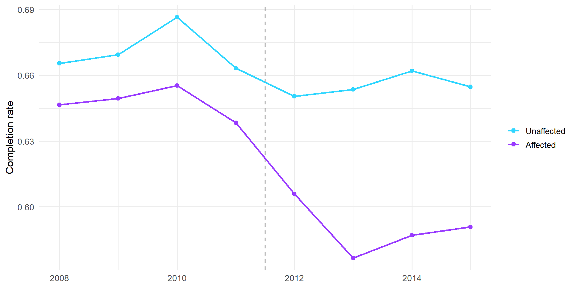

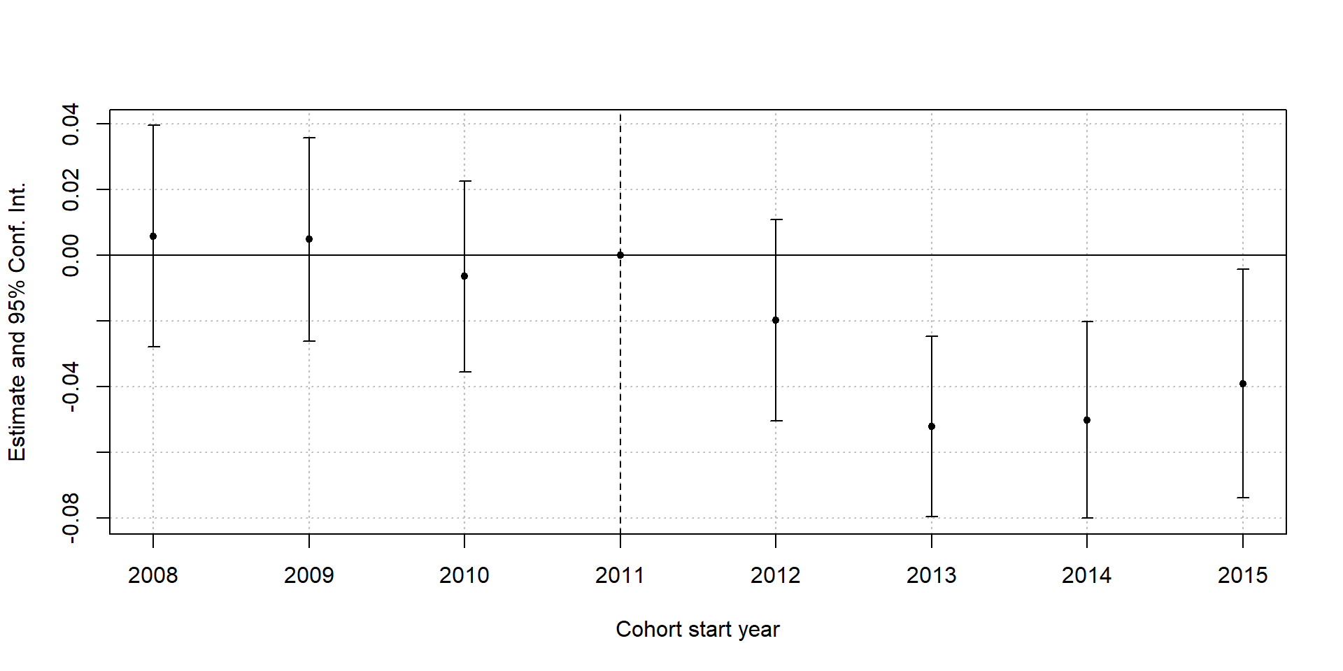
• TIME — 6 min
• Four pre-reform years, and the two lines move broadly together. That is the assumption we need
• “Broadly together” is doing work. Take two or three of the sentences people wrote — it is a judgement, not a test
• The levels differ, and that is fine. Difference-in-differences requires parallel trends, not equal levels
• Push back on anyone who says the pre-period looks perfectly flat. It does not, and a dataset where it did would be suspicious

Parallel trends, formally

What should the pre-reform coefficients look like if the assumption holds — and what would you conclude if one were significant?

es <- feols(
    completion ~ i(start_year, affected, ref = 2011) |
        framework_id + start_year,
    data = panel, cluster = ~framework_id
)

iplot(es, main = "", xlab = "Cohort start year")

• TIME — 12 min
• The event study puts a confidence interval on the eyeball judgement. Pre-reform coefficients sit close to zero and none is individually significant
• 2011 is the reference year, so it has no coefficient by construction — worth stating, people always ask
• The post-reform coefficients are consistently negative and of similar size: an effect that appears at the reform and persists, rather than one drifting in beforehand
• If a pre-period coefficient had been large and significant, the DiD would not be credible and no amount of controls would fix it
• The i() syntax is on screen because nobody guesses it: variable, interacted with, reference level

Four outcomes, one specification

Aim: the same two-way fixed effects model for four outcomes, clustered by framework — with the earnings model weighted by the number of completers behind each cell mean.

What do the framework and year fixed effects absorb? Why are there no sector or level controls? And why does the earnings model carry weights when the others do not?

m_starts <- feols(log(starts) ~ did | framework_id + start_year,
    data = panel, cluster = ~framework_id
)
m_comp <- feols(completion ~ did | framework_id + start_year,
    data = panel, cluster = ~framework_id
)
m_ach <- feols(achievement ~ did | framework_id + start_year,
    data = panel, cluster = ~framework_id
)
m_earn <- feols(log_earn ~ did | framework_id + start_year,
    data = panel, weights = ~n_earn, cluster = ~framework_id
)

etable(m_starts, m_comp, m_ach, m_earn, digits = 3, fitstat = ~n)

#>                          m_starts            m_comp             m_ach           m_earn
#> Dependent Var.:       log(starts)        completion       achievement         log_earn
#>                                                                                       
#> did             -0.168*** (0.016) -0.041*** (0.008) -0.052*** (0.009) 0.064*** (0.007)
#> Fixed-Effects:  ----------------- ----------------- ----------------- ----------------
#> framework_id                  Yes               Yes               Yes              Yes
#> start_year                    Yes               Yes               Yes              Yes
#> _______________ _________________ _________________ _________________ ________________
#> S.E.: Clustered  by: framework_id  by: framework_id  by: framework_id by: framework_id
#> Observations                  640               640               640              640
#> ---
#> Signif. codes: 0 '***' 0.001 '**' 0.01 '*' 0.05 '.' 0.1 ' ' 1

• TIME — 14 min
• Read across: starts fall around 17%, completion about 4 percentage points, achievement about 5, and earnings among completers rise about 6%
• Framework fixed effects absorb everything time-invariant about a framework — sector, level, typical learner. Year fixed effects absorb anything hitting all frameworks at once, like the recession
• Clustering at the framework: 80 clusters, comfortably enough, and a nice callback to this morning
• Note we did not need sector or level controls. The framework fixed effects already absorb them — a good test of whether people have understood what fixed effects do
• The weights. A regression on cell means asks: is each cell one observation, or is it a stand-in for the people in it? For starts the cell is the unit. For earnings the cells are means over completers with a PAYE record, and the reform changed how many of those there are in exactly the treated cells — so unweighted, the affected post-reform cells count for more per person than everyone else. Unweighted gives 0.055; weighted by completers gives 0.064, which is what you get from the 65,863 individual rows. Have them try it
• For completion and achievement the same choice moves the estimate by a few thousandths, because every cell has at least 40 starts and the reform did not change who counts as a starter. Weighting is the honest default whenever the cells are different sizes; it just happens to matter here only for earnings

Fewer complete, yet completers earn more

Fewer people start. Fewer complete. Fewer achieve.

And yet those who do complete earn more.

Discussion in threes — 5 minutes

What is going on? Give me two competing explanations, and say what you would look at to tell them apart.

• TIME — 10 min
• Let this run. It is the best discussion of the day and the room usually gets both answers between them
• Explanation 1, optimistic: longer apprenticeships with more guided learning genuinely build more skill, so completers are worth more to employers
• Explanation 2, deflationary: the reform pushed out the marginal apprentices. Those who still complete are a more able, more committed group than before, so average earnings rise even if nobody learned anything extra. Composition, not causation
• Both are consistent with the coefficients as reported. Distinguishing them needs individual characteristics or a bound on selection
• Do not resolve it yet — the next slide does

Composition or a real earnings gain?

Aim: by group and period, the share of starters who reach the earnings sample, and the prior attainment of those who do.

starts |>
    left_join(framework_pre, by = "framework_id") |>
    mutate(
        period = ifelse(start_year >= 2012, "Post", "Pre"),
        group = ifelse(affected == 1, "Affected", "Unaffected")
    ) |>
    group_by(group, period) |>
    summarise(
        starts = n(),
        pct_with_earnings = round(100 * mean(!is.na(earnings_12m)), 1),
        prior_of_earners = round(mean(as.numeric(prior_attain)[!is.na(earnings_12m)],
            na.rm = TRUE
        ), 2),
        .groups = "drop"
    )

#> # A tibble: 4 × 5
#>   group      period starts pct_with_earnings prior_of_earners
#>   <chr>      <chr>   <int>             <dbl>            <dbl>
#> 1 Affected   Post    29295              49.6            10.2 
#> 2 Affected   Pre     31938              54.6             9.94
#> 3 Unaffected Post    30553              57.1            10.7 
#> 4 Unaffected Pre     28215              58.2            10.4

• The people we observe earning changed: the share reaching the earnings sample falls 5 points in affected frameworks, 1 point elsewhere
• But their observable prior attainment moves the same in both groups
• In the data we built, the true direct effect on earnings is +0.062. The plain 2×2 gives +0.070, so about +0.008 — a tenth, not a fifth — is composition, on things you cannot see

• TIME — 10 min
• This is the reveal, and it is only possible because we constructed the data. In a real study you could not decompose it this cleanly — which is exactly why the interpretation question is hard in practice
• So the optimistic story is mostly right here, and a tenth of the headline is selection. The selection is on the unobserved propensity to complete, which is why prior attainment does not show it — and why, in real data, a balance table on observables would not settle the argument
• The practical lesson: whenever a policy changes who ends up in your analysis sample, an outcome measured on that sample is partly about composition. Conditioning on a post-treatment variable — completion — is the specific sin
• A cleaner alternative is earnings for everyone who STARTED. Ask why we did not lead with that: it dilutes the effect across people who never finished, and answers a different question. It is in the appendix

Robustness: does the specification matter?

Aim: the plain 2×2 interaction on the same panel, with the same weights, beside the two-way fixed effects model.

When would the two disagree — and why should they agree here?

simple <- feols(log_earn ~ affected * post,
    data = panel,
    weights = ~n_earn, cluster = ~framework_id
)

etable(simple, m_earn, digits = 4, fitstat = ~n)

#>                              simple             m_earn
#> Dependent Var.:            log_earn           log_earn
#>                                                       
#> Constant          9.697*** (0.0452)                   
#> affected            0.0521 (0.0625)                   
#> post            -0.0237*** (0.0049)                   
#> affected x post  0.0700*** (0.0072)                   
#> did                                 0.0641*** (0.0065)
#> Fixed-Effects:  ------------------- ------------------
#> framework_id                     No                Yes
#> start_year                       No                Yes
#> _______________ ___________________ __________________
#> S.E.: Clustered    by: framework_id   by: framework_id
#> Observations                    640                640
#> ---
#> Signif. codes: 0 '***' 0.001 '**' 0.01 '*' 0.05 '.' 0.1 ' ' 1

• The plain 2×2 and the two-way fixed effects model agree to within a standard error
• Expected here: a single national reform date means no staggered adoption, so the two-way fixed effects problems from Module 3 do not arise

• TIME — 6 min
• Be explicit: the Goodman-Bacon and Callaway-Sant’Anna critiques are about treatment timing varying across units. With one common date there are no forbidden comparisons and TWFE is fine
• 0.070 against 0.064: the fixed effects soak up level differences between frameworks that the 2×2 leaves in the error, and the small gap is that
• So this is a case where the sophisticated estimator is unnecessary, and knowing when you do not need it is as useful as knowing how to run it
• The did package would give essentially the same answer. Not running it live because it is slow and adds nothing here

Robustness: a placebo reform

Pairs — 5 minutes

Pretend the reform happened in 2011 instead. Using only pre-reform years, is there an effect on completion?

panel |>
    filter(start_year < 2012) |>
    mutate(
        fake_post = as.integer(start_year >= 2011),
        fake_did = affected * fake_post
    ) |>
    feols(completion ~ fake_did | framework_id + start_year,
        data = _, cluster = ~framework_id
    ) |>
    coeftable() |>
    round(4)

#>          Estimate Std. Error t value Pr(>|t|)
#> fake_did  -0.0014     0.0123 -0.1178   0.9065
#> attr(,"type")
#> [1] "Clustered (framework_id)"

• TIME — 9 min
• A null result here is the good outcome, and it takes people a moment to accept that
• If a fake reform date produced an effect, the two groups were already diverging and our real estimate was picking up that trend rather than the policy
• A genuinely useful test to run on any DiD, and it costs three lines
• Pairs that finish early: the appendix has the near-threshold and by-sector checks

Reporting this to a policy audience

Finding	Magnitude	Confidence
Starts	Down ~17%	Very high
Completion rate	Down ~4pp	High
Achievement rate	Down ~5pp	High
Earnings of completers	Up ~6%	High, but partly composition

• Lead with the trade-off, not with one number: the reform raised quality per apprenticeship and reduced volume
• Whether that is a good deal depends on what the programme is for — a political question, not a statistical one

• TIME — 10 min
• Push the room. Report only the earnings result and you have misled the reader; report only the fall in starts and you have done the same in the other direction
• The honest framing is the trade-off, with the composition caveat attached to the earnings figure
• Ask what a Minister would ask next. Usually: how many fewer apprentices in absolute numbers, and what happened to those who did not start
• That last question is the one this design cannot answer, and saying so is the mark of a good evaluator

Exercise 2: what you did

• Defined treatment from pre-reform data only, so the reform could not define its own treated group
• Checked the policy actually changed behaviour before looking at any outcome
• Built a panel, assessed parallel trends by eye and with an event study
• Estimated four outcomes with one specification, weighted the one whose cells changed size, and read them together
• Found a result that looked like an unambiguous success, and took it apart
• Ran a placebo, and saw why a null there is the good outcome

If you are ahead — four extensions in the appendix: frameworks near the 12-month threshold, effects by sector, earnings for everyone who started, and an event study on earnings.

• TIME — 3 min
• Ninety seconds, then the break. Same shape as the morning: estimand, design check, estimate, attack your own result

Exercise 3: Regression Discontinuity

Born a day apart

England admits children to school by a 1 September cutoff.

• A child born 31 August is the youngest in their cohort
• A child born 1 September is the oldest in the next one

Two children born a day apart are near-identical in every respect except where they sit in their year group — and that is assigned by a date nobody chose with schooling in mind.

The question: does being young for your year affect attainment, and identification of special educational needs?

• TIME — 3 min
• This is the classic UK application of RDD and it is worth thirty seconds on why it is compelling: the running variable is date of birth, which is recorded precisely and cannot be manipulated after the fact
• Crawford, Dearden and Meghir (2010) and Crawford, Dearden and Greaves (2013) are the England references, both on the NPD. The striking figure: August-born girls are around 72% more likely to be identified with non-statemented SEN at age 11 than September-born girls
• Flag now that we will come back to what exactly this design identifies, because it is less obvious than it looks — but let them find the discontinuity first
• If time is short this is the exercise we compress. The core is the running variable, the density test, the plot and the estimate; the bins and robustness slides can be shown rather than run, and the appendix is never presented anyway

Build the running variable

cohort <- read_csv("data/npd_cohort.csv", show_col_types = FALSE)
dim(cohort)

#> [1] 80000     9

names(cohort)

#> [1] "pupil_id"      "date_of_birth" "cohort_year"   "gender"        "ethnic"       
#> [6] "fsm6"          "idaci_rank"    "ks2_score"     "sen_support"

On your own — 5 minutes

Build the running variable: days from 1 September, negative for children born before it and zero or positive for those born on or after. Check its range, and the share on each side.

cutoff <- as.Date("2009-09-01")
cohort <- cohort |>
    mutate(
        days = as.integer(date_of_birth - cutoff),
        after = as.integer(days >= 0)
    )

range(cohort$days)

#> [1] -182  181

mean(cohort$after)

#> [1] 0.470725

• TIME — 7 min
• It is deliberately the first thing they do, because in a real RDD constructing and sanity-checking the running variable is most of the work
• The centring matters: the threshold must sit at zero, or every package you hand it will estimate the jump in the wrong place
• Watch for anyone treating date_of_birth as character — read_csv parses it as a Date, but a read.csv user will get a string and silently produce nonsense. This is the trap promised on the “awkward bits” slide
• cohort_year is in the file so nobody has to reconstruct academic-year membership from a date. That is a data management exercise, not an RDD one

Before anything else: can people sort themselves?

Aim: test for a jump in the density of the running variable at zero.

Predict first: what would manipulation look like in a histogram of birth dates?

library(rddensity)
dens <- rddensity(cohort$days, c = 0, bino = FALSE)
summary(dens)

#> 
#> Manipulation testing using local polynomial density estimation.
#> 
#> Number of obs =       80000
#> Model =               unrestricted
#> Kernel =              triangular
#> BW method =           estimated
#> VCE method =          jackknife
#> 
#> c = 0                 Left of c           Right of c          
#> Number of obs         42342               37658               
#> Eff. Number of obs    10970               9308                
#> Order est. (p)        2                   2                   
#> Order bias (q)        3                   3                   
#> BW est. (h)           46.957              40.505              
#> 
#> Method                T                   P > |T|             
#> Robust                0.9539              0.3401

• If parents could time births to land the right side of 1 September, the children either side would no longer be comparable

• TIME — 4 min
• Run this first, before any plot of the outcome. It is the assumption everything else rests on, and running it last is how people talk themselves into a result
• The test should NOT reject here, and that is the teaching point on the next slide. Do not preview it — let them see the histogram first and draw the wrong conclusion
• bino = FALSE switches off the package’s binomial tests in small windows around the cutoff. With a running variable in whole days those windows are asymmetric — one day on the left against two on the right — so every one of them “rejects” at p = 0.000 for no reason at all. Anyone who runs the default at home will see that table; tell them why it is off
• There is a real literature on birth timing around school cutoffs, mostly finding small effects at the margin for elective deliveries. Worth mentioning as the reason this test is not merely ceremonial

Non-uniform is not the same as manipulated

ggplot(cohort, aes(days)) +
    geom_histogram(binwidth = 7, fill = "#993bff", alpha = 0.8) +
    geom_vline(xintercept = 0, linetype = "dashed") +
    labs(x = "Days from 1 September", y = "Births")

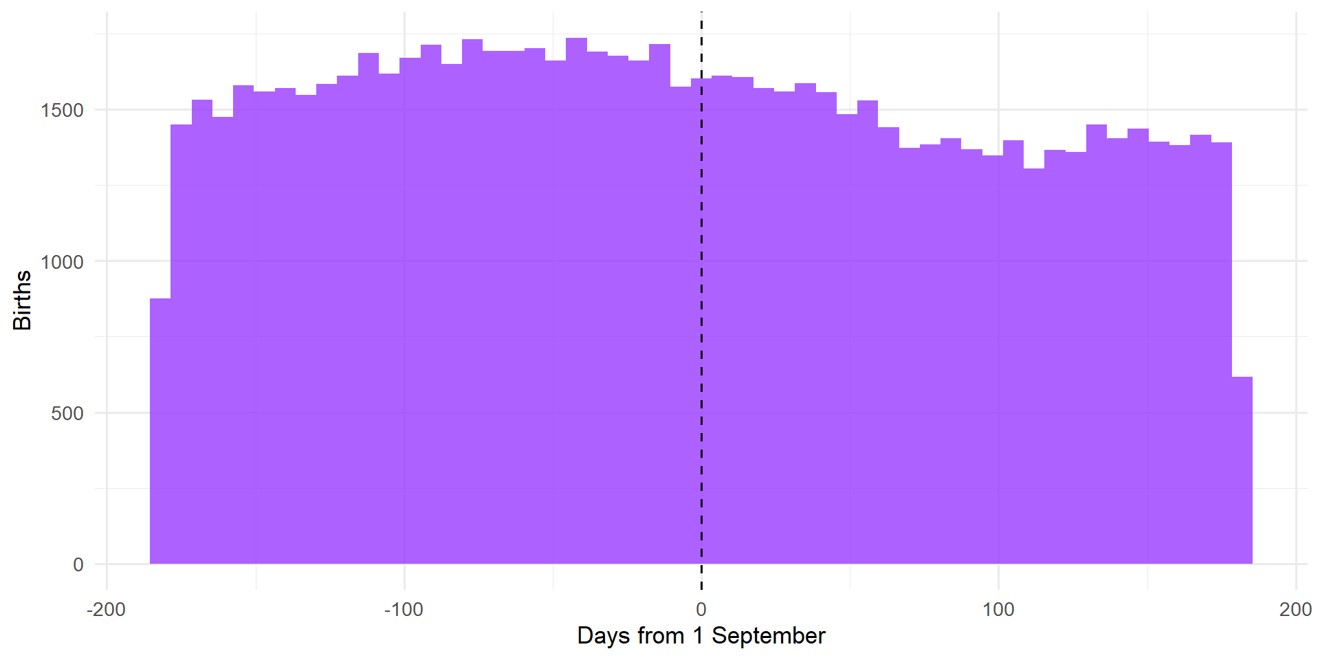
• The distribution is visibly not flat — births peak in late summer, as they really do
• But there is no step at the threshold, and a step is the only thing that would threaten the design

• TIME — 3 min
• This is the slide worth protecting time for. Almost everyone looks at that histogram and says “that is not uniform, the design is broken” — and they are wrong
• The test is for a discontinuity AT the cutoff, not for uniformity anywhere. A smooth seasonal cycle is exactly what you would expect from real births and is no threat at all
• The same confusion turns up in covariate balance checks: people test whether a covariate is related to the running variable, when the question is whether it jumps at the threshold
• If someone asks how you would spot real manipulation: look for a spike in the last few days before the cutoff and a hole just after, which is what date-of-birth reporting fraud looks like

Plot the discontinuity

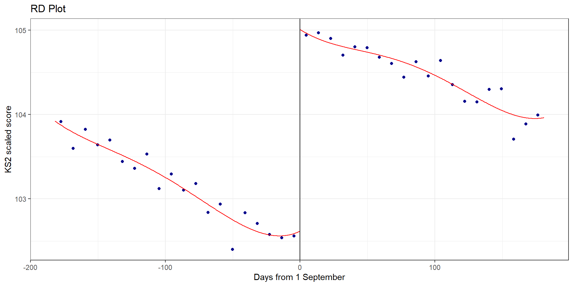
Aim: the mean KS2 score in bins of the running variable, either side of the cutoff, with a fitted line on each side.

Two things to read off: the jump at zero, and the slope within each side. What is the slope?

library(rdrobust)
rdplot(
    y = cohort$ks2_score, x = cohort$days, c = 0,
    nbins = c(20, 20),
    x.label = "Days from 1 September", y.label = "KS2 scaled score"
)

• TIME — 5 min
• Let them sit with the picture before anyone estimates anything. If you cannot see it here, no amount of bandwidth selection will rescue it
• Two things to draw out. First the jump at zero, which is the effect. Second the DOWNWARD slope within each side, which is the same phenomenon operating continuously: the later in the cohort year you are born, the younger you are relative to your peers
• That sawtooth is the signature of a relative age effect and is worth naming — it is what tells you the discontinuity is not an artefact of something happening on 1 September for unrelated reasons
• Ask what the slope would look like if being young for your year did not matter: flat, with no step

Bins: too few, too many

for (b in c(4, 20, 80, 182)) {
    print(rdplot(cohort$ks2_score, cohort$days,
        c = 0, nbins = c(b, b), hide = TRUE,
        title = paste(b, "bins per side"), x.label = "", y.label = ""
    )$rdplot)
}

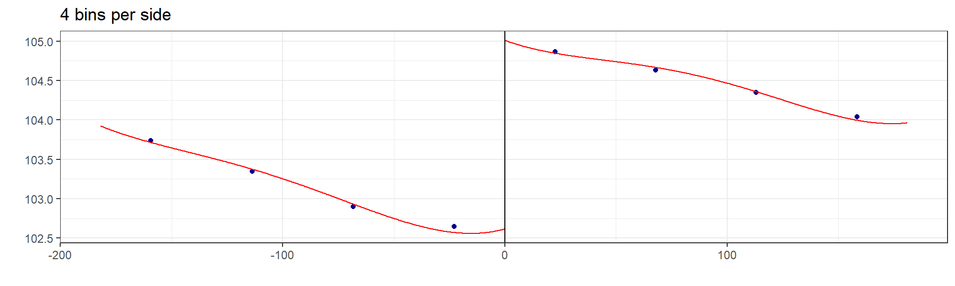
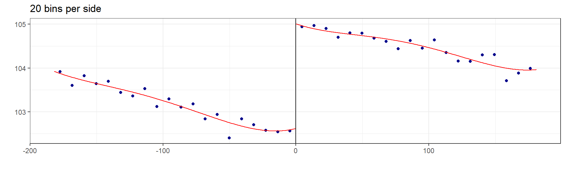
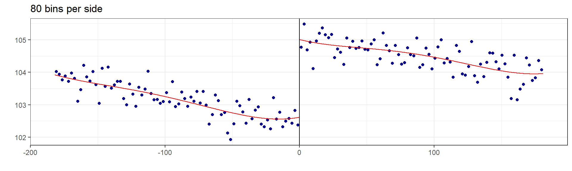
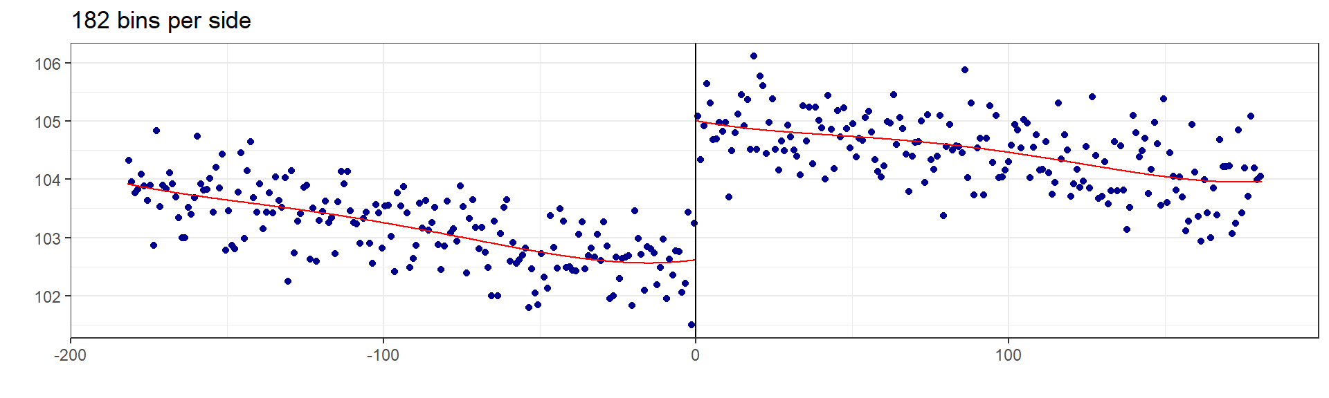
• 4 bins: the jump is there, but four points tell you nothing about the noise, and the fitted curve is doing all the work
• 182 bins (one per day): honest about the noise, hard to read
• 20 is a choice, not a fact. rdplot’s default picks the number that mimics the variance of the raw data. A bin must never straddle the cutoff

• TIME — 3 min
• Module 4’s bin-width point, made with the same data. Too wide hides how much noise there is and lets the fitted curve carry the picture; too narrow is all noise
• The one rule that is not a matter of taste: no bin straddles the cutoff, or the jump gets averaged away. rdplot bins each side separately for exactly this reason
• The default binselect is data-driven and picks a number close to one bin per day here. That is fine for the estimate and useless for a policy audience; the plot you publish is a communication choice, and you say what you chose

Local linear estimate at the cutoff

Which of the three rows do you report, and why?

fit <- rdrobust(y = cohort$ks2_score, x = cohort$days, c = 0)
summary(fit, all = TRUE)

#> Call: rdrobust
#> 
#> Sharp RD estimates using local polynomial regression.
#> 
#> Number of Obs.                80000
#> BW type                       mserd
#> Kernel                   Triangular
#> VCE method                       NN
#> 
#>                                Left        Right
#> Number of Obs.                42342        37658
#> Eff. Number of Obs.           15796        14862
#> Order est. (p)                    1            1
#> Order bias (q)                    2            2
#> BW est. (h)                  66.108       66.108
#> BW bias (b)                 107.568      107.568
#> rho (h/b)                     0.615        0.615
#> Unique Obs.                     182          182
#> 
#> =======================================================================================
#>         Method     Coef. Std. Err.         z     P>|z|      [ 95% C.I. ]       
#> =======================================================================================
#>   Conventional     2.425     0.175    13.878     0.000     [2.083 , 2.768]     
#> Bias-Corrected     2.377     0.175    13.601     0.000     [2.034 , 2.719]     
#>         Robust     2.377     0.206    11.555     0.000     [1.974 , 2.780]     
#> =======================================================================================

• Local linear regression either side of the cutoff, weighted by a triangular kernel so points nearest the threshold count most
• The bandwidth is chosen by the data, not by you — report which one, and why

• TIME — 5 min
• Read the output together. Three rows: conventional, bias-corrected, and robust. Report the robust one; it is the whole point of the package and its interval is wider for a good reason. Conventional ignores the smoothing bias; bias-corrected subtracts an estimate of it (from the local quadratic at bandwidth b) but keeps the conventional SE; robust also widens the SE for the noise in that bias estimate
• all = TRUE is there because rdrobust 4.0 prints one row by default: the conventional point estimate with the robust interval, which is why that interval is not centred on the estimate. Someone will spot it
• The bandwidth line matters as much as the estimate. rdrobust selects an MSE-optimal bandwidth by default and it comes out at 66 days, about two months either side. A CER-optimal bandwidth (bwselect = "cerrd") is narrower and is the one to prefer if the interval matters more than the point estimate
• The estimate is 2.4 scaled score points, comfortably significant with 80,000 pupils. In SD terms that is roughly a third of a standard deviation, which is large for anything in education
• Note what is NOT in the model: no covariates. Adjustment in an RDD buys precision, never identification, and if adding covariates moves the point estimate you have a problem rather than a better answer. The appendix checks it

Bandwidth sensitivity and covariate placebos

Aim: the estimate at half and double the chosen bandwidth; then the same estimator with FSM and IDACI as the outcome.

## Halve and double the data-driven bandwidth
h <- fit$bws[1, 1]
for (b in c(h / 2, h, h * 2)) {
    r <- rdrobust(cohort$ks2_score, cohort$days, c = 0, h = b)
    cat(sprintf(
        "h = %5.1f days   est = %6.3f   p = %.4f\n",
        b, r$coef[1], r$pv[3]
    ))
}

#> h =  33.1 days   est =  2.353   p = 0.0000

#> h =  66.1 days   est =  2.425   p = 0.0000

#> h = 132.2 days   est =  2.542   p = 0.0000

## Covariates must NOT jump at the cutoff
for (v in c("fsm6", "idaci_rank")) {
    r <- rdrobust(cohort[[v]], cohort$days, c = 0)
    cat(sprintf("%-12s est = %9.3f   p = %.3f\n", v, r$coef[1], r$pv[3]))
}

#> fsm6         est =     0.008   p = 0.356

#> idaci_rank   est =   -50.280   p = 0.736

• TIME — 5 min
• Bandwidth sensitivity first: the estimate should move a little and the conclusion not at all. If halving the bandwidth halves the effect, the functional form is doing the work rather than the discontinuity
• Then the covariate placebos. FSM and deprivation are determined long before a child starts school, so they cannot jump at the cutoff. If they do, something is wrong with the design or the data
• These should pass, and participants need to see what passing looks like — most published examples people meet are the ones where a check failed
• Placebo cutoffs, a different polynomial order and a donut are in the appendix

SEN identification at the cutoff

Aim: the same estimator with SEN support as the outcome.

Which direction do you expect — and so what sign will the coefficient carry?

rdrobust(cohort$sen_support, cohort$days, c = 0) |> summary()

#> Call: rdrobust
#> 
#> Sharp RD estimates using local polynomial regression.
#> 
#> Number of Obs.                80000
#> BW type                       mserd
#> Kernel                   Triangular
#> VCE method                       NN
#> 
#>                                Left        Right
#> Number of Obs.                42342        37658
#> Eff. Number of Obs.           12403        11891
#> Order est. (p)                    1            1
#> Order bias (q)                    2            2
#> BW est. (h)                  52.306       52.306
#> BW bias (b)                  81.590       81.590
#> rho (h/b)                     0.641        0.641
#> Unique Obs.                     182          182
#> 
#> =====================================================================
#>                    Point    Robust Inference
#>                 Estimate         z     P>|z|      [ 95% C.I. ]       
#> ---------------------------------------------------------------------
#>      RD Effect    -0.041    -3.830     0.000    [-0.064 , -0.021]    
#> =====================================================================

• Children who are youngest in their cohort are more likely to be identified as having special educational needs
• Same date of birth, same child — different position in the year group, different chance of being labelled

• TIME — 3 min
• The sign question is real: the jump is measured going from left (youngest, August-born) to right (oldest, September-born), so a negative coefficient means the oldest are less likely to be identified — 4 percentage points lower, on a base of 12%
• This is the finding worth ending the substantive part on, because it is the one with immediate policy bite. It is not that August-born children have more need; it is that need is judged relative to classmates who are up to a year older
• Crawford, Dearden and Greaves put the effect at around 72% higher odds for August-born girls at age 11. Ours is the same phenomenon in percentage points
• Ask the room what should follow from it. Age-standardised assessment is the obvious answer, and the honest response is that it is harder than it sounds

What did you actually identify?

Across 1 September, three things change at once:

• Relative age — youngest in the cohort becomes oldest in the next
• Absolute age at test — the September-born child sits KS2 nearly a year older
• The year the test is sat — a different cohort, a different paper, a different school year

The design identifies their combined effect. It cannot separate them.

This is why the published literature decomposes date-of-birth effects rather than reporting a single cutoff estimate.

• TIME — 4 min
• Do not skip this, even if you are short of time — cut a robustness slide instead. Estimating the discontinuity is the easy half; knowing what it is an estimate OF is the job
• Work through why the three are inseparable here. Anyone born just before the cutoff is in the earlier cohort by definition, so you cannot hold cohort fixed and vary relative age. The design gives you the bundle
• The literature separates them using variation across cohorts and across countries with different cutoffs, plus policy changes in the cutoff date itself. That is a much bigger exercise than one regression
• The general lesson, which applies to every RDD: the estimand is whatever changes discontinuously at the threshold — all of it, not just the bit you are interested in. Ask what else moves at your cutoff
• Good closing question for the room: if you were advising a minister on summer-born children, which of the three would you actually want to know about?

Exercise 3: what you did

• Built and centred a running variable, and checked it before touching an outcome
• Tested for manipulation, and learned that non-uniform is not the same as manipulated
• Looked before estimating, and saw why the bins are a choice
• Estimated a local linear jump, and reported the right row
• Checked bandwidth sensitivity and covariate smoothness, and saw what passing looks like
• Worked out what the discontinuity is actually an estimate of

If you are ahead — four extensions in the appendix: placebo cutoffs, a different polynomial and kernel, covariates and a donut, and the estimate by gender.

• TIME — 3 min
• Ninety seconds, then wrap-up. If this exercise was cut, this slide is still worth showing: it is the map of what the solution script does

Wrap-Up

What you did today

• Checked the data you were sent matched the design you were told about — and found two schools missing
• Estimated an ITT effect and watched covariate adjustment change the conclusion
• Clustered standard errors at the level of randomisation, and saw what ignoring that would have cost
• Distinguished attrition that is non-random from attrition that is differential
• Built a panel, assessed parallel trends, ran an event study and a placebo test
• Found a result that looked like an unambiguous success, and took it apart
• Found a discontinuity, checked nobody could sort across it, and then worked out what it was actually an estimate of

• TIME — 6 min
• Reinforce that the hardest parts today were not the models. feols and rdrobust are one line each; deciding what belongs in them, and what the number means afterwards, is the job
• All three exercises share a shape: work out what you are estimating, check the design held, estimate it, then attack your own result
• If Exercise 3 was cut for time, say so and point them at the solution script — it runs standalone and the slides are in the deck they are taking away

Taking it further

Everything from today

• Slides, the data, the solution scripts and the generator that made the data are all in the workshop repository — take the folder with you
• The code you wrote today keeps working, because the data is not going anywhere
• The appendix has twelve extensions, all with working code

Where to go next

• The online modules cover the theory in more depth: Module 2 for the morning, Module 3 for the afternoon, Module 4 for the last exercise
• For real data: ADR UK for administrative data access, the ONS Secure Research Service for LEO itself

• TIME — 5 min
• Worth saying explicitly that the data ships with the folder, because people expect a licence hurdle and there isn’t one. They can hand it to a colleague, use it in their own teaching, or keep practising on it
• build-workshop-data.R is in there too. Nobody needs to run it, but anyone curious about how the effects were set can read it, and the parameters are all named constants near the top of each exercise
• The step up to real data is governance, not code. The techniques today transfer directly; what changes is the months of application beforehand and the output checking afterwards
• Invite questions afterwards

Thank you

Jake Anders, Oliver Cassagneau-Francis, Fabien Petit UCL Centre for Education Policy & Equalising Opportunities

ADR Evaluation Extension

• TIME — 4 min
• Final questions
• Feedback form, if there is one

Appendix: If You Are Ahead

Exercise 1: the pre-specified subgroup

Aim: interact treatment with FSM eligibility in the adjusted model. Anders et al. pre-specified FSM as the primary subgroup; everything else was exploratory.

Why an interaction rather than two separate regressions?

feols(attainment8 ~ arm * fsm6 + ks2_score + sen_support + eal | block,
    data = analysis, cluster = ~school_urn
) |>
    coeftable() |>
    (\(x) round(x[grepl("arm", rownames(x)), ], 3))()

#>                   Estimate Std. Error t value Pr(>|t|)
#> armtreatment         2.098      0.848   2.475    0.015
#> armtreatment:fsm6   -0.782      0.794  -0.985    0.326

• No evidence the effect differs by FSM status: the interaction is small, negative, and nowhere near significant
• One pre-specified subgroup is a test. Twelve post-hoc subgroups is a fishing expedition

• Never presented. An interaction gives the difference between subgroups with a standard error; two separate regressions give two estimates and no test of the difference
• Back to Exercise 1

Exercise 1: multiple imputation with mice

Aim: impute the 673 missing KS2 scores five times, with treatment arm in the imputation model, fit the adjusted model on each, and pool with Rubin’s rules.

library(mice)
imp_dat <- analysis |>
    select(attainment8, arm, ks2_score, fsm6, sen_support, eal, idaci_rank) |>
    mutate(arm = factor(arm))
imp <- mice(imp_dat, m = 5, method = "pmm", seed = 1, printFlag = FALSE)

fits <- lapply(1:5, \(i) {
    complete(imp, i) |>
        mutate(school_urn = analysis$school_urn, block = analysis$block) |>
        feols(attainment8 ~ arm + ks2_score + fsm6 + sen_support + eal | block,
            data = _, cluster = ~school_urn
        )
})

## Rubin's rules by hand, because pool() does not know about clustered fixest models
est <- sapply(fits, \(f) coef(f)[["armtreatment"]])
v <- sapply(fits, \(f) se(f)[["armtreatment"]]^2)
round(c(
    estimate = mean(est), se = sqrt(mean(v) + (1 + 1 / 5) * var(est)),
    complete_case = coef(m3)[["armtreatment"]], cc_se = se(m3)[["armtreatment"]]
), 3)

#>      estimate            se complete_case         cc_se 
#>         1.884         0.798         1.887         0.804

• Nothing changes. With 2.7% of a covariate missing and the outcome complete, imputation cannot add much
• The point is the workflow: arm in the imputation model, pool properly, and keep the clustering

• Never presented. Runs in about two seconds on this data
• pool(with(imp, lm(...))) is the textbook route and it works — but it drops the clustering and reports a standard error a quarter of the right size. Which is the reason to do Rubin by hand here
• Back to Exercise 1

Exercise 1: randomisation inference

Aim: re-randomise treatment across schools within blocks 200 times, refit, and place the observed estimate in that null distribution.

schools_arm <- analysis |> distinct(school_urn, block, arm)
observed <- coef(m3)[["armtreatment"]]

set.seed(20260910)
null <- replicate(200, {
    fake <- schools_arm |>
        group_by(block) |>
        mutate(arm = sample(arm)) |>
        ungroup()
    d <- analysis |>
        select(-arm) |>
        left_join(fake, by = c("school_urn", "block"))
    coef(feols(attainment8 ~ arm + ks2_score + fsm6 + sen_support + eal | block,
        data = d
    ))[["armtreatment"]]
})

round(c(
    observed = observed, p_randomisation = mean(abs(null) >= abs(observed)),
    p_model = pvalue(m3)[["armtreatment"]]
), 3)

#>        observed p_randomisation         p_model 
#>           1.887           0.015           0.020

• The randomisation p-value needs no asymptotics and no assumption about the error structure — it uses only the fact that assignment was random
• It agrees with the clustered p-value here, because 138 clusters is plenty. With 12 local authorities it would not, and this is the one to trust

• Never presented. About seven seconds; 500 permutations would be better for a report
• Permuting within block is the point: re-randomise the way the trial randomised
• Back to Exercise 1

Exercise 1: are the models on the same sample?

Aim: refit the unadjusted model on the pupils the adjusted model actually used. Is the gap between 1.31 and 1.89 adjustment, or a different sample?

feols(attainment8 ~ arm,
    data = filter(analysis, !is.na(ks2_score)),
    cluster = ~school_urn
) |>
    coeftable() |>
    (\(x) round(x["armtreatment", ], 3))()

#>   Estimate Std. Error    t value   Pr(>|t|) 
#>      1.310      1.571      0.834      0.406

• The unadjusted estimate on the common sample is close to the full-sample one: the difference is adjustment, not composition
• Worth doing in any report where covariates carry missingness

• Never presented. A one-line check that is routinely skipped
• Back to Exercise 1

Exercise 2: frameworks near the threshold

Aim: restrict to frameworks whose pre-reform duration was between 9 and 15 months, where affected and unaffected are most alike, and re-estimate completion and earnings.

The appendix works on the individual rows (ind) rather than the panel: with weights they give the same answers, and the subsetting is easier to read.

ind <- starts |>
    left_join(framework_pre, by = "framework_id") |>
    mutate(post = as.integer(start_year >= 2012), did = affected * post)

near <- ind |> filter(duration_pre > 9, duration_pre < 15)
n_distinct(near$framework_id)

#> [1] 34

near_comp <- feols(completion ~ did | framework_id + start_year,
    data = near, cluster = ~framework_id
)
near_earn <- feols(log(earnings_12m) ~ did | framework_id + start_year,
    data = near, cluster = ~framework_id
)
etable(near_comp, near_earn, digits = 3, fitstat = ~n)

#>                         near_comp         near_earn
#> Dependent Var.:        completion log(earnings_12m)
#>                                                    
#> did             -0.048*** (0.007)     0.034 (0.034)
#> Fixed-Effects:  ----------------- -----------------
#> framework_id                  Yes               Yes
#> start_year                    Yes               Yes
#> _______________ _________________ _________________
#> S.E.: Clustered  by: framework_id  by: framework_id
#> Observations               53,706            27,131
#> ---
#> Signif. codes: 0 '***' 0.001 '**' 0.01 '*' 0.05 '.' 0.1 ' ' 1

• Completion holds up. The earnings effect is the same size but no longer significant: 34 clusters, and the interval has doubled
• A robustness check that “fails” on power rather than on sign is not a failure, and you say so

• Never presented. The near-threshold comparison is the one a sceptical referee asks for, and it is where a regression discontinuity on duration would start
• Back to Exercise 2

Exercise 2: effects by sector

Aim: the completion effect separately for the five largest sector subject areas, in one model.

frameworks <- read_csv("data/framework_lookup.csv", show_col_types = FALSE)
ind_sector <- ind |>
    left_join(select(frameworks, framework_id, ssa_tier1), by = "framework_id")
top5 <- ind_sector |>
    count(ssa_tier1, sort = TRUE) |>
    slice_head(n = 5) |>
    pull(ssa_tier1)

feols(completion ~ did:ssa_tier1 | framework_id + start_year,
    data = filter(ind_sector, ssa_tier1 %in% top5), cluster = ~framework_id
) |>
    coeftable() |>
    (\(x) round(x[, 1:2], 3))()

#>                                                               Estimate Std. Error
#> did:ssa_tier1Business, Administration and Law                   -0.046      0.014
#> did:ssa_tier1Construction, Planning and the Built Environment   -0.043      0.006
#> did:ssa_tier1Engineering and Manufacturing Technologies         -0.031      0.015
#> did:ssa_tier1Leisure, Travel and Tourism                        -0.046      0.004
#> did:ssa_tier1Retail and Commercial Enterprise                   -0.047      0.007

• Every sector’s completion rate fell by three to five points. The effect is not being carried by one sector
• Sector is in the framework lookup, not the starts file: a join you would have to do in the ILR too

• Never presented. did:ssa_tier1 without a main effect for sector, because the framework fixed effects already absorb it
• Back to Exercise 2

Exercise 2: earnings for everyone who started

Aim: earnings in pounds, counting non-completers and those without a PAYE record as zero, for every start.

feols(coalesce(earnings_12m, 0) ~ did | framework_id + start_year,
    data = ind, cluster = ~framework_id
) |>
    coeftable() |>
    round(2)

#>     Estimate Std. Error t value Pr(>|t|)
#> did   -97.65     125.21   -0.78     0.44
#> attr(,"type")
#> [1] "Clustered (framework_id)"

• Nothing: about −£100 on a base of £10,300, with an interval that spans zero comfortably
• Higher earnings for completers and fewer completers cancel out. This answers a different question — what did the reform do to the earnings of a person who started — and it is the question a Treasury analyst would ask

• Never presented. Zeros for non-completers is one convention; earnings conditional on any employment is another. Say which
• Back to Exercise 2

Exercise 2: an event study on earnings

Aim: the event study from the main flow, on log earnings at the individual level.

es_earn <- feols(
    log(earnings_12m) ~ i(start_year, affected, ref = 2011) |
        framework_id + start_year,
    data = ind, cluster = ~framework_id
)

iplot(es_earn, main = "", xlab = "Cohort start year")

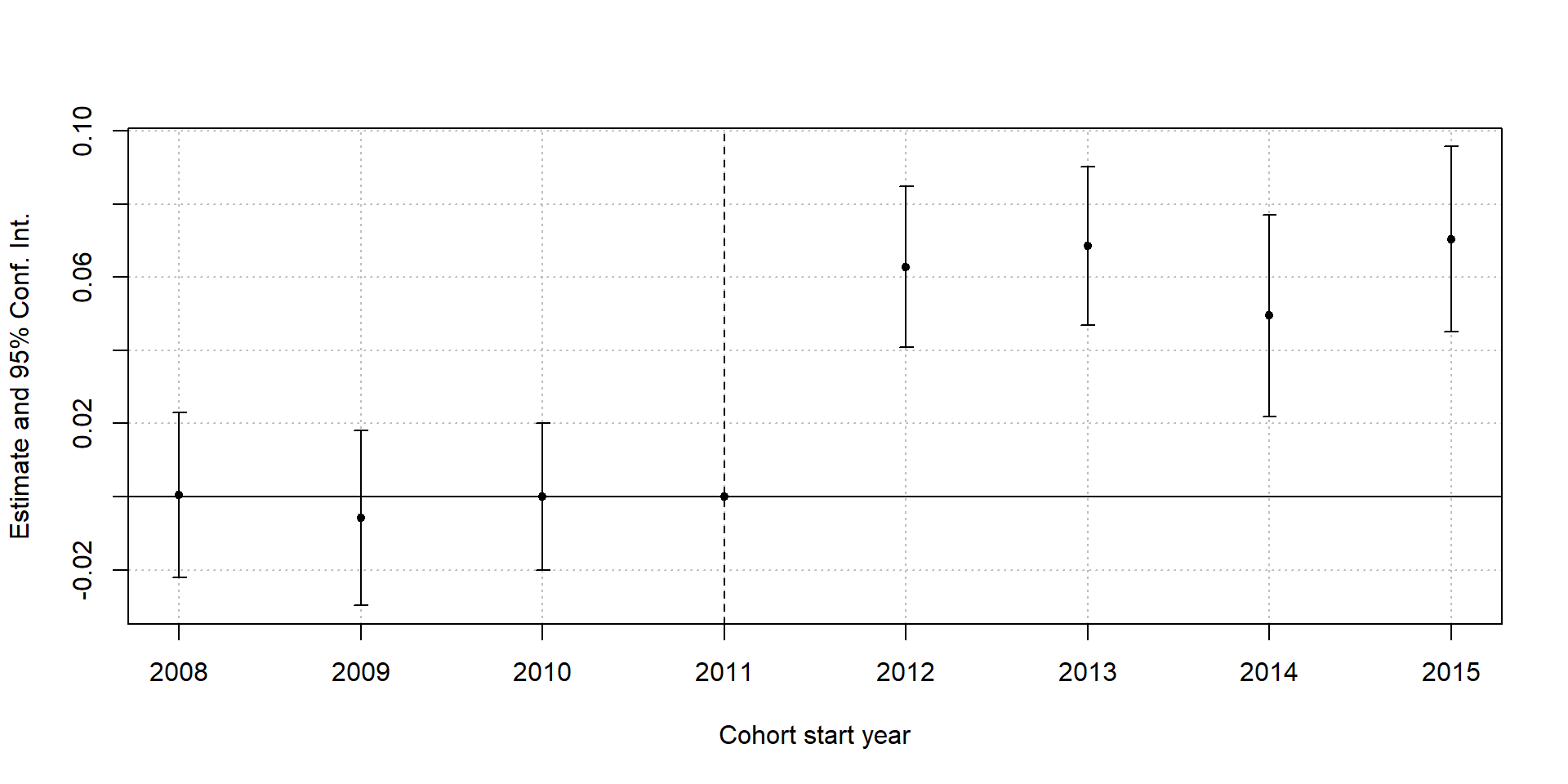
• Flat before, a step of five to seven log points after, and no drift in either direction
• The same check as for completion, and it should be run for every outcome you report

• Never presented
• Back to Exercise 2

Exercise 3: placebo cutoffs

Aim: estimate the “jump” 120 days either side of the real cutoff — early May and late December, where nothing happens — using only the side of the real cutoff each sits on.

for (fake in c(-120, 120)) {
    side <- cohort |> filter(sign(days) == sign(fake))
    r <- rdrobust(side$ks2_score, side$days, c = fake)
    cat(sprintf(
        "cutoff at %+4d days   est = %6.3f   p = %.3f\n",
        fake, r$coef[1], r$pv[3]
    ))
}

#> cutoff at -120 days   est =  0.417   p = 0.142

#> cutoff at +120 days   est = -0.456   p = 0.262

• Nothing at either placebo, against 2.4 points at the real one
• Restricting to one side matters: a placebo window that spans the real cutoff would pick up the real jump

• Never presented
• Back to Exercise 3

Exercise 3: polynomial order and kernel

Aim: the same estimate with a local quadratic, and with a uniform kernel.

for (spec in list(
    list(p = 2, kernel = "triangular"),
    list(p = 1, kernel = "uniform")
)) {
    r <- rdrobust(cohort$ks2_score, cohort$days, c = 0, p = spec$p, kernel = spec$kernel)
    cat(sprintf(
        "p = %d  %-10s   h = %5.1f   est = %.3f   p = %.3f\n",
        spec$p, spec$kernel, r$bws[1, 1], r$coef[1], r$pv[3]
    ))
}

#> p = 2  triangular   h =  88.2   est = 2.364   p = 0.000

#> p = 1  uniform      h =  40.5   est = 2.467   p = 0.000

• A quadratic chooses a wider bandwidth and lands within a tenth of a point; the uniform kernel chooses a narrower one and does the same
• Local linear with a triangular kernel is the default for a reason, and these are the two checks Module 4 asks for

• Never presented. Higher-order polynomials over the full support are the thing to avoid (Gelman and Imbens); a local quadratic within the bandwidth is fine as a check
• Back to Exercise 3

Exercise 3: covariates and a donut

Aim: add FSM, IDACI and gender as covariates; then drop the three days either side of the cutoff and re-estimate.

with_covs <- rdrobust(cohort$ks2_score, cohort$days,
    c = 0,
    covs = cbind(cohort$fsm6, cohort$idaci_rank, cohort$gender == "F")
)
donut <- cohort |> filter(abs(days) > 3)
with_donut <- rdrobust(donut$ks2_score, donut$days, c = 0)

tibble(
    spec = c("Baseline", "With covariates", "Donut ±3 days"),
    estimate = c(fit$coef[1], with_covs$coef[1], with_donut$coef[1]),
    se = c(fit$se[3], with_covs$se[3], with_donut$se[3])
) |>
    mutate(across(where(is.numeric), \(x) round(x, 3)))

#> # A tibble: 3 × 3
#>   spec            estimate    se
#>   <chr>              <dbl> <dbl>
#> 1 Baseline            2.42 0.206
#> 2 With covariates     2.44 0.194
#> 3 Donut ±3 days       2.49 0.261

• Covariates tighten the standard error a little and move the estimate not at all — which is what a valid design looks like
• The donut is for suspected manipulation right at the cutoff. Nothing here suggests it, and the estimate does not care

• Never presented. If covariates had moved the estimate, that is evidence the covariates jump at the cutoff — a design problem, not a better answer
• Back to Exercise 3

Exercise 3: by gender

Aim: the KS2 and SEN discontinuities separately for girls and boys. The published finding is largest for girls.

for (g in c("F", "M")) {
    s <- cohort |> filter(gender == g)
    ks2 <- rdrobust(s$ks2_score, s$days, c = 0)
    sen <- rdrobust(s$sen_support, s$days, c = 0)
    cat(sprintf(
        "%s   KS2 jump = %.2f (p = %.3f)   SEN jump = %.3f (p = %.3f)\n",
        g, ks2$coef[1], ks2$pv[3], sen$coef[1], sen$pv[3]
    ))
}

#> F   KS2 jump = 2.11 (p = 0.000)   SEN jump = -0.041 (p = 0.012)

#> M   KS2 jump = 2.70 (p = 0.000)   SEN jump = -0.038 (p = 0.003)

• Here the KS2 jump is larger for boys and the SEN jump is the same for both — which tells you about our simulation, not about children
• Subsample checks are Module 4’s last robustness item, and the honest use of them is to report all of them, not the one that looks best

• Never presented. We did not build a gender difference into the discontinuity, so any gap here is noise; the published girls result comes from real data
• Back to Exercise 3